Hevitra ato Anatiny
10th day of the marathon 30 Excel miasa ao anatin'ny 30 andro we will devote to the study of the function HLOOKUP (GPR). This feature is very similar to VLOOKUP (VLOOKUP), only it works with elements of a horizontal list.
Unfortunate function HLOOKUP (GLOW) is not as popular as its sister, since in most cases the data in the tables is arranged vertically. Remember the last time you wanted to search for a string? What about returning the value from the same column, but located in one of the rows below?
Anyway, let’s give features HLOOKUP (GPR) a well-deserved moment of glory and take a closer look at the information about this feature, as well as examples of its use. Remember, if you have interesting ideas or examples, please share them in the comments.
Function 10: HLOOKUP
asa HLOOKUP (HLOOKUP) looks up the value in the first row of the table and returns another value from the same column in the table.
How can I use the HLOOKUP (HLOOKUP) function?
Hatramin'ny asa HLOOKUP (HLOOKUP) can find an exact or approximate value in a string, then it can:
- Find sales totals for the selected region.
- Find an indicator that is relevant for the selected date.
HLOOKUP Syntax
asa HLOOKUP (HLOOKUP) has the following syntax:
HLOOKUP(lookup_value,table_array,row_index_num,range_lookup)
ГПР(искомое_значение;таблица;номер_строки;интервальный_просмотр)
- lookup_value (lookup_value): Ny sanda ho hita. Mety ho sanda na fanondro sela.
- table_array (table): lookup table. Can be a range reference or a named range containing 2 lines or more.
- row_index_num (line_number): A string containing the value to be returned by the function. Set by the row number within the table.
- range_lookup (range_lookup): Use FALSE or 0 to find an exact match; for an approximate search, TRUE (TRUE) or 1. In the latter case, the string in which the function is searching must be sorted in ascending order.
Traps HLOOKUP (GPR)
toy ny VLOOKUP (VLOOKUP), function HLOOKUP (HLOOKUP) can be slow, especially when searching for an exact match of a text string in an unsorted table. Whenever possible, use an approximate search in a table sorted by the first row in ascending order. You can first apply the function lalao (Miharihary kokoa) na COUNTIF (COUNTIF) to make sure the value you’re looking for even exists in the first row.
Ny endri-javatra hafa toy ny INDEX (INDEX) ary lalao (MATCH) dia azo ampiasaina haka soatoavina avy amin'ny latabatra ary mahomby kokoa. Hojerentsika any aoriana any amin'ny hazakazaka ataontsika izy ireo ary hojerentsika hoe hatraiza ny heriny sy ny fahaizany.
Example 1: Find sales values for a selected region
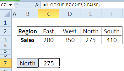
Mamelà ahy hampahatsiahy anao indray fa ny asa HLOOKUP (HLOOKUP) only looks for the value in the top row of the table. In this example, we will find the sales totals for the selected region. It is important for us to get the correct value, so we use the following settings:
- The region name is entered in cell B7.
- The regional lookup table has two rows and spans the range C2:F3.
- The sales totals are in row 2 of our table.
- The last argument is set to FALSE to find an exact match when searching.
Ny formula ao amin'ny cell C7 dia:
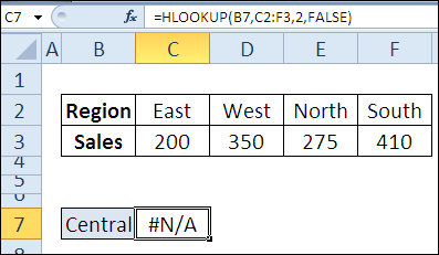
=HLOOKUP(B7,C2:F3,2,FALSE)
=ГПР(B7;C2:F3;2;ЛОЖЬ)
If the name of the region is not found in the first row of the table, the result of the function HLOOKUP (GPR) will #AT (#N / A).
Example 2: Find a measure for a selected date
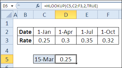
Matetika rehefa mampiasa ny asa HLOOKUP (HLOOKUP) requires an exact match, but sometimes an approximate match is more appropriate. For example, if the indicators change at the beginning of each quarter, and the first days of these quarters are used as column headings (see the figure below). In this case, using the function HLOOKUP (HLOOKUP) and an approximate match, you will find an indicator that is relevant for a given date. In this example:
- The date is written in cell C5.
- The indicator lookup table has two rows and is located in the range C2:F3.
- The lookup table is sorted by date row in ascending order.
- The indicators are recorded in line 2 of our table.
- The function’s last argument is set to TRUE to look for an approximate match.
The formula in cell D5 is:
=HLOOKUP(C5,C2:F3,2,TRUE)
=ГПР(C5;C2:F3;2;ИСТИНА)
If the date is not found in the first row of the table, the function HLOOKUP (HLOOKUP) will find the nearest largest value that is less than the argument lookup_value (lookup_value). In this example, the desired value is Marsa 15. It is not in the date line, so the formula will take the value 1 Janoary ary hiverina 0,25.